All works shown here are created using genuine mathematical algorithms written in Python.
In the mathematics of dynamical systems, an attractor is a set of values towards which a system naturally evolves over time, effectively acting like a "magnet" for the system's behaviour.
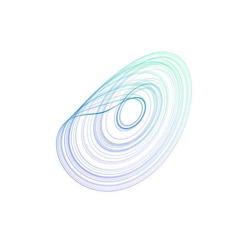 System: Chaos Theory (Continuous ODE)
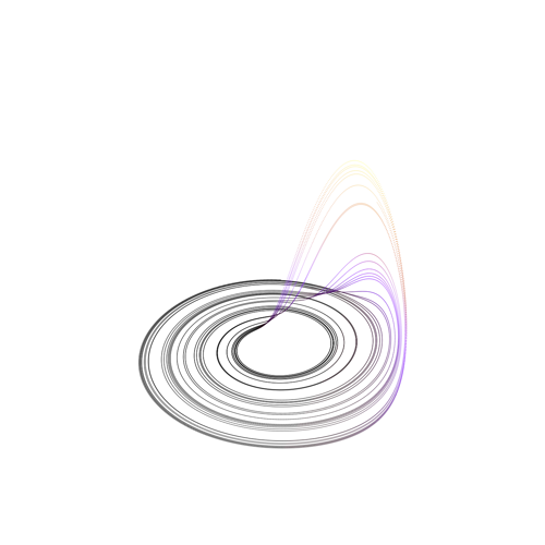 System: Chaos Theory (Continuous ODE)
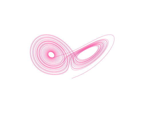 System: Chaos Theory (Continuous ODE)
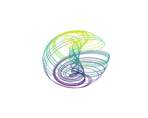 System: Chaos Theory (Continuous ODE)
 System: Chaos Theory (Continuous ODE)
 System: Chaos Theory (Continuous ODE)
Parametric curves are geometric shapes defined by equations where each coordinate is a function of a single independent variable (often "t"), allowing for the description of complex, self-intersecting paths that standard functions cannot model.
 System: 2D Parametric Curve
 System: 2D Parametric Curve
 System: Maurer Rose (Parametric)
 System: 2D Parametric Curve
 System: 2D Parametric Curve
 System: Damped Parametric (Harmonograph)
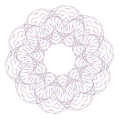 System: 2D Parametric Curve (Guilloché)
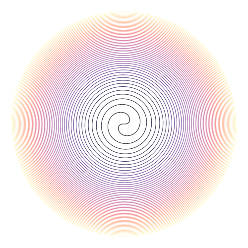 System: 2D Parametric Curve
Fractals are infinitely complex patterns created by repeating a simple equation in a feedback loop, resulting in shapes that look the same at any scale (self-similarity).
 System: 2D Fractal (Iterated Function System)
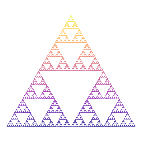 System: 2D Fractal (Chaos Game)
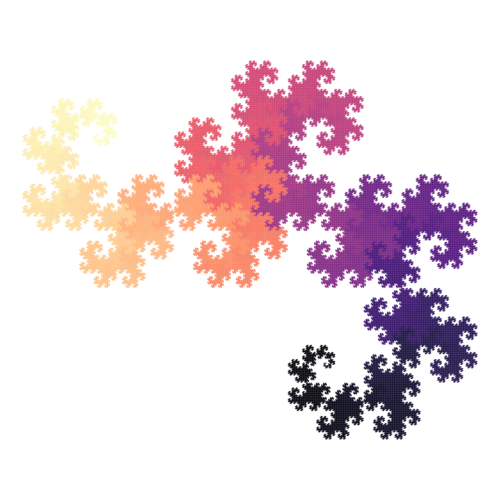 System: 2D Fractal (Iterated Function System / L-System)
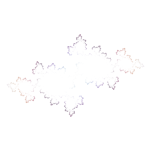 System: 2D Fractal (Inverse Iteration Method)
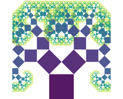 System: 2D Fractal (Geometric Recursion)
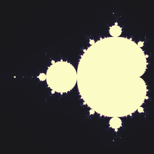 System: 2D Fractal (Complex Dynamics)
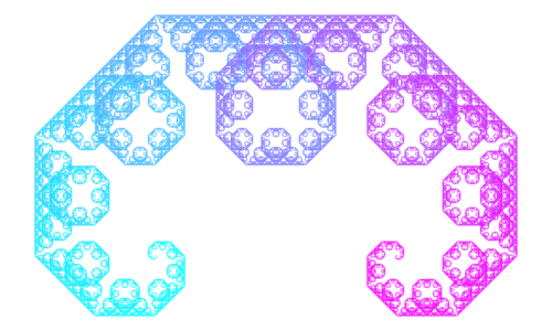 System: 2D Fractal (Iterated Function System)
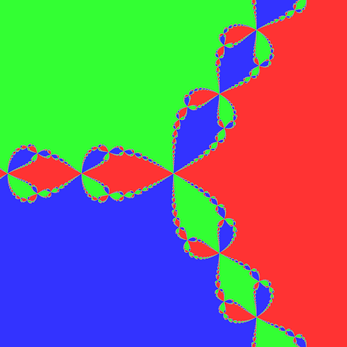 System: 2D Fractal (Complex Dynamics)
Tessellations are patterns formed by repeating geometric shapes to cover a surface completely without any gaps or overlaps.
 System: 3D Tessellation
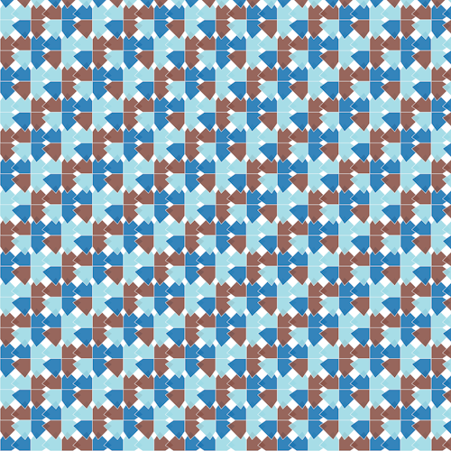 System: 2D Tessellation
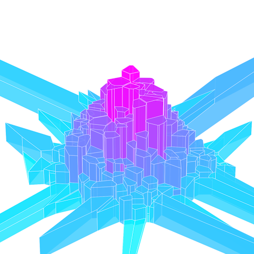 System: 3D Tessellation
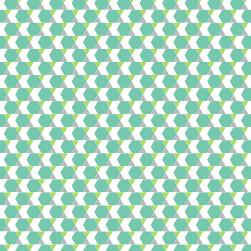 System: 2D Tessellation
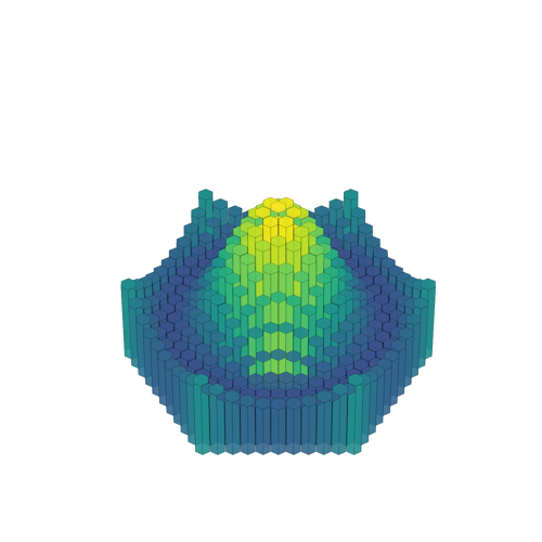
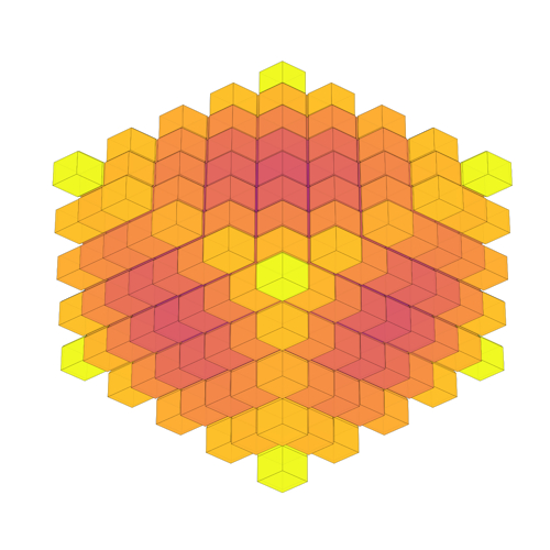 System: 3D Tessellation (Space Filling)
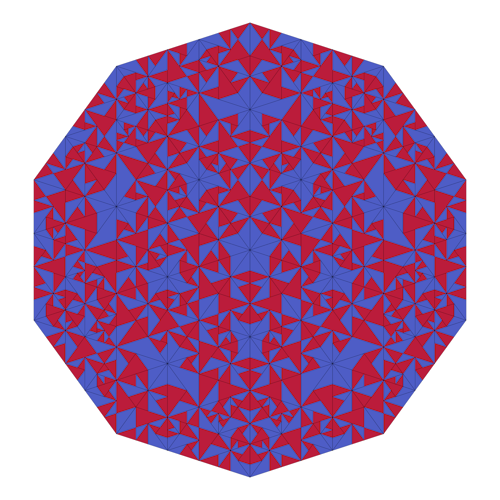 System: 2D Tessellation (Aperiodic)
A minimal surface is a shape that naturally finds the most efficient way to stretch across a boundary, using the least amount of surface area possible.
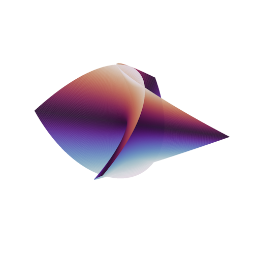 System: Minimal Surface (Differential Geometry)
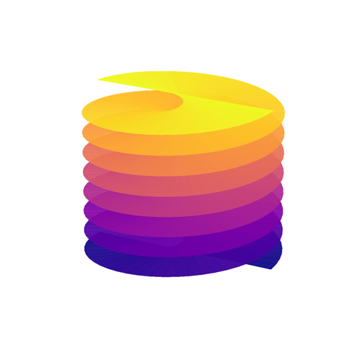 System: Minimal Surface (Ruled Surface)
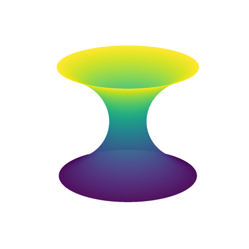 System: Minimal Surface (Surface of Revolution)
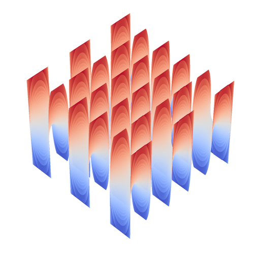 System: Minimal Surface (Doubly Periodic)
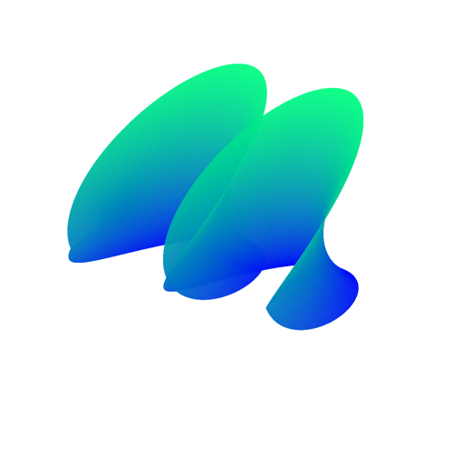 System: Minimal Surface
 System: Minimal Surface (Non-orientable)
© 2025 elliptica • All rights reserved • Powered by the 3 pillars of web design • HTML, CSS and JS